Sample Splitting with Caret/SuperLearner • evalITR

Train the model with Caret

We can train the model with the caret package (for further information about caret, see the original website). We use parallel computing to speed up the computation.

# parallel computing
library(doParallel)
cl <- makePSOCKcluster(5)
registerDoParallel(cl)

# stop after finishing the computation
stopCluster(cl)

The following example shows how to estimate the ITR with gradient boosting machine (GBM) using the caret package. Note that we have already loaded the data and specify the treatment, outcome, and covariates as shown in the Sample Splitting vignette. Since we are using the caret package, we need to specify the trainControl and/or tuneGrid arguments. The trainControl argument specifies the cross-validation method and the tuneGrid argument specifies the tuning grid. For more information about these arguments, please refer to the caret website.

We estimate the ITR with only one machine learning algorithm (GBM) and evaluate the ITR with the evaluate_itr() function. To compute PAPDp, we need to specify the algorithms argument with more than 2 machine learning algorithms.

library(evalITR)
library(caret)

# specify the trainControl method
fitControl <- caret::trainControl(
  method = "repeatedcv", # 3-fold CV
  number = 3, # repeated 3 times
  repeats = 3,
  search='grid',
  allowParallel = TRUE) # grid search

# specify the tuning grid
gbmGrid <- expand.grid(
  interaction.depth = c(1, 5, 9), 
  n.trees = (1:30)*50, 
  shrinkage = 0.1,
  n.minobsinnode = 20)

# estimate ITR
fit_caret <- estimate_itr(
  treatment = "treatment",
  form = user_formula,
  trControl = fitControl,
  data = star_data,
  algorithms = c("gbm"),
  budget = 0.2,
  split_ratio = 0.7,
  tuneGrid = gbmGrid,
  verbose = FALSE)
#> Evaluate ITR under sample splitting ...

# evaluate ITR
est_caret <- evaluate_itr(fit_caret)
#> Cannot compute PAPDp

We can extract the training model from caret and check the model performance. Other functions from caret can be applied to the training model.

# extract the final model
caret_model <- fit_caret$estimates$models$gbm
print(caret_model$finalModel)
#> A gradient boosted model with gaussian loss function.
#> 100 iterations were performed.
#> There were 53 predictors of which 24 had non-zero influence.

# check model performance
trellis.par.set(caretTheme()) # theme
plot(caret_model)

# heatmap 
plot(
  caret_model, 
  plotType = "level",
  scales = list(x = list(rot = 90)))

Train the model with SuperLearner

Alternatively, we can train the model with the SuperLearner package (for further information about SuperLearner, see the original website). SuperLearner utilizes ensemble method by taking optimal weighted average of multiple machine learning algorithms to improve model performance.

We will compare the performance of the ITR estimated with causal_forest and SuperLearner.

library(SuperLearner)

fit_sl <- estimate_itr(
  treatment = "treatment",
  form = user_formula,
  data = star_data,
  algorithms = c("causal_forest","SuperLearner"),
  budget = 0.2,
  split_ratio = 0.7,
  SL_library = c("SL.ranger", "SL.glmnet"))
#> Evaluate ITR under sample splitting ...

est_sl <- evaluate_itr(fit_sl)

# summarize estimates
summary(est_sl)
#> -- PAPE ------------------------------------------------------------------------
#>   estimate std.deviation     algorithm statistic p.value
#> 1      1.9           1.4 causal_forest       1.4    0.17
#> 2      2.3           1.4  SuperLearner       1.6    0.11
#> 
#> -- PAPEp -----------------------------------------------------------------------
#>   estimate std.deviation     algorithm statistic p.value
#> 1      1.8           1.1 causal_forest       1.6   0.112
#> 2      2.1           1.2  SuperLearner       1.8   0.071
#> 
#> -- PAPDp -----------------------------------------------------------------------
#>   estimate std.deviation                    algorithm statistic p.value
#> 1     -0.3          0.97 causal_forest x SuperLearner     -0.31    0.76
#> 
#> -- AUPEC -----------------------------------------------------------------------
#>   estimate std.deviation     algorithm statistic p.value
#> 1      1.5           1.0 causal_forest       1.5    0.14
#> 2      1.6           1.1  SuperLearner       1.5    0.14
#> 
#> -- GATE ------------------------------------------------------------------------
#>    estimate std.deviation     algorithm group statistic p.value upper lower
#> 1      -172           107 causal_forest     1     -1.61    0.11  -347     4
#> 2      -145           108 causal_forest     2     -1.35    0.18  -323    32
#> 3       102           109 causal_forest     3      0.94    0.35   -76   281
#> 4       142           109 causal_forest     4      1.31    0.19   -37   321
#> 5       103           108 causal_forest     5      0.95    0.34   -76   281
#> 6       -59           108  SuperLearner     1     -0.55    0.58  -237   118
#> 7       -79           107  SuperLearner     2     -0.73    0.46  -255    98
#> 8        36           109  SuperLearner     3      0.33    0.74  -143   214
#> 9        28           108  SuperLearner     4      0.26    0.79  -150   207
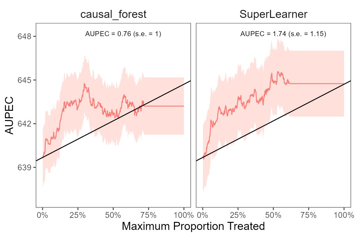
#> 10      104           109  SuperLearner     5      0.95    0.34   -75   283

We plot the estimated Area Under the Prescriptive Effect Curve for the writing score across a range of budget constraints, seperately for the two ITRs, estimated with causal_forest and SuperLearner.

# plot the AUPEC 
plot(est_sl)