Cross-validation with multiple ML algorithms
Source:vignettes/cv_multiple_alg.Rmd
cv_multiple_alg.RmdWe can estimate ITR with various machine learning algorithms and then
compare the performance of each model. The package includes all ML
algorithms in the caret package and 2 additional algorithms
(causal
forest and bartCause).
The package also allows estimate heterogeneous treatment effects on
the individual and group-level. On the individual-level, the summary
statistics and the AUPEC plot show whether assigning individualized
treatment rules may outperform complete random experiment. On the
group-level, we specify the number of groups through ngates
and estimating heterogeneous treatment effects across groups.
library(evalITR)
#> Loading required package: MASS
#>
#> Attaching package: 'MASS'
#> The following object is masked from 'package:dplyr':
#>
#> select
#> Loading required package: Matrix
#> Loading required package: quadprog
# specify the trainControl method
fitControl <- caret::trainControl(
method = "repeatedcv",
number = 3,
repeats = 3)
# estimate ITR
set.seed(2021)
fit_cv <- estimate_itr(
treatment = "treatment",
form = user_formula,
data = star_data,
trControl = fitControl,
algorithms = c(
"causal_forest",
"bartc",
# "rlasso", # from rlearner
# "ulasso", # from rlearner
"lasso", # from caret package
"rf"
), # from caret package
budget = 0.2,
n_folds = 3)
#> Evaluate ITR with cross-validation ...
#> Loading required package: lattice
#> Loading required package: ggplot2
#> fitting treatment model via method 'bart'
#> fitting response model via method 'bart'
#> fitting treatment model via method 'bart'
#> fitting response model via method 'bart'
#> fitting treatment model via method 'bart'
#> fitting response model via method 'bart'
# evaluate ITR
est_cv <- evaluate_itr(fit_cv)
#>
#> Attaching package: 'purrr'
#> The following object is masked from 'package:caret':
#>
#> lift
# summarize estimates
summary(est_cv)
#> -- PAPE ------------------------------------------------------------------------
#> estimate std.deviation algorithm statistic p.value
#> 1 0.27 0.82 causal_forest 0.33 0.74
#> 2 -0.09 0.66 bartc -0.14 0.89
#> 3 0.17 1.07 lasso 0.16 0.87
#> 4 1.27 0.95 rf 1.33 0.18
#>
#> -- PAPEp -----------------------------------------------------------------------
#> estimate std.deviation algorithm statistic p.value
#> 1 2.32 0.68 causal_forest 3.39 0.0007
#> 2 1.71 1.07 bartc 1.59 0.1123
#> 3 -0.21 0.63 lasso -0.33 0.7406
#> 4 1.69 1.11 rf 1.52 0.1287
#>
#> -- PAPDp -----------------------------------------------------------------------
#> estimate std.deviation algorithm statistic p.value
#> 1 0.609 0.63 causal_forest x bartc 0.960 0.3371
#> 2 2.524 0.80 causal_forest x lasso 3.145 0.0017
#> 3 0.631 0.73 causal_forest x rf 0.859 0.3906
#> 4 1.914 1.00 bartc x lasso 1.916 0.0554
#> 5 0.022 1.35 bartc x rf 0.016 0.9873
#> 6 -1.893 0.72 lasso x rf -2.615 0.0089
#>
#> -- AUPEC -----------------------------------------------------------------------
#> estimate std.deviation algorithm statistic p.value
#> 1 1.23 1.6 causal_forest 0.79 0.43
#> 2 0.86 1.4 bartc 0.60 0.55
#> 3 0.18 1.4 lasso 0.13 0.90
#> 4 1.37 1.6 rf 0.88 0.38
#>
#> -- GATE ------------------------------------------------------------------------
#> estimate std.deviation algorithm group statistic p.value upper lower
#> 1 -110.1 59 causal_forest 1 -1.871 0.061 5.2 -225
#> 2 45.8 59 causal_forest 2 0.771 0.441 162.2 -71
#> 3 101.7 59 causal_forest 3 1.721 0.085 217.6 -14
#> 4 -38.1 74 causal_forest 4 -0.519 0.604 106.0 -182
#> 5 18.9 95 causal_forest 5 0.199 0.843 205.7 -168
#> 6 21.2 62 bartc 1 0.343 0.732 142.6 -100
#> 7 -127.1 59 bartc 2 -2.151 0.031 -11.3 -243
#> 8 -1.1 97 bartc 3 -0.011 0.991 189.8 -192
#> 9 82.0 59 bartc 4 1.390 0.165 197.6 -34
#> 10 43.2 95 bartc 5 0.457 0.648 228.8 -142
#> 11 -14.4 94 lasso 1 -0.154 0.878 169.2 -198
#> 12 -94.5 90 lasso 2 -1.051 0.293 81.8 -271
#> 13 87.9 99 lasso 3 0.886 0.376 282.4 -107
#> 14 12.6 59 lasso 4 0.214 0.830 127.8 -103
#> 15 26.6 59 lasso 5 0.451 0.652 142.4 -89
#> 16 -37.4 59 rf 1 -0.638 0.523 77.5 -152
#> 17 10.6 59 rf 2 0.180 0.857 126.5 -105
#> 18 -17.6 59 rf 3 -0.299 0.765 97.7 -133
#> 19 66.5 86 rf 4 0.770 0.441 235.9 -103
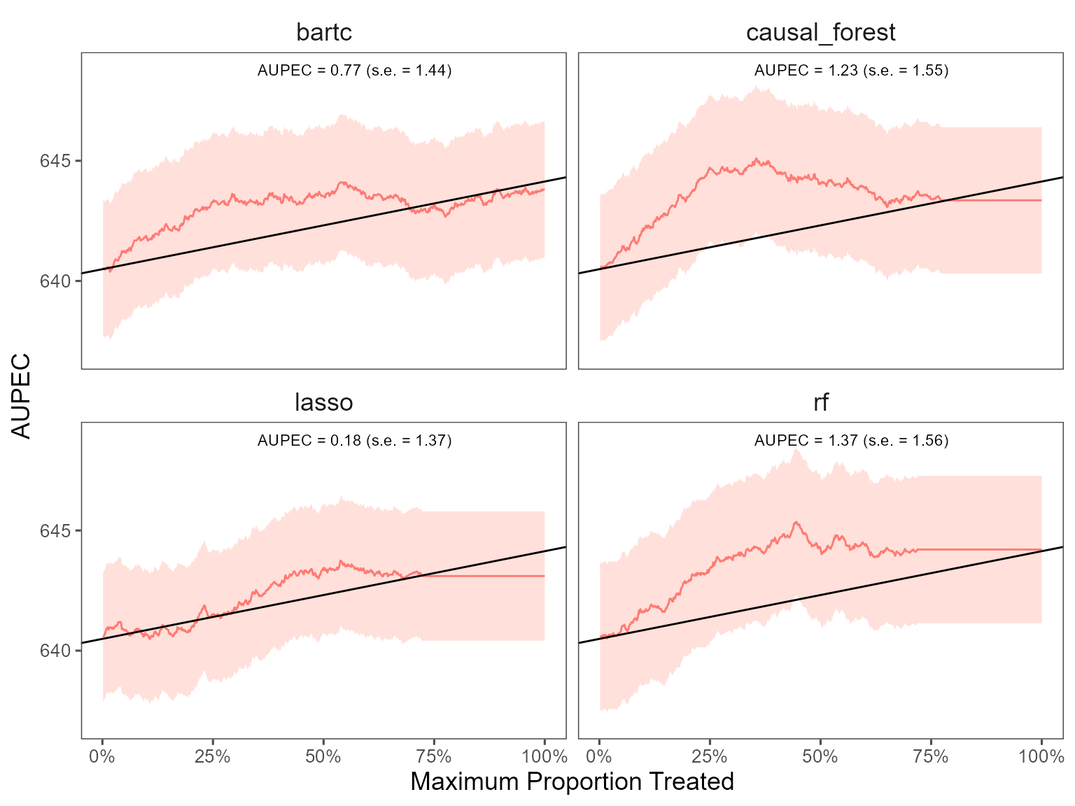
#> 20 -3.9 60 rf 5 -0.066 0.948 113.0 -121We plot the estimated Area Under the Prescriptive Effect Curve for the writing score across different ML algorithms.
# plot the AUPEC with different ML algorithms
plot(est_cv)